Image Data Representations

This example demonstrates how to use points_to_cells() and cells_to_points() to re-mesh ImageData.

These filters can be used to ensure that image data has an appropriate representation when generating plots and/or when using either point- or cell-based filters such as ImageDataFilters.image_threshold (point-based) and DataSetFilters.threshold (cell-based).

Representations of 3D Volumes

Create image data of a 3D volume with eight points and a discrete scalar data array.

from __future__ import annotations

import numpy as np

import pyvista as pv



data_array = [8, 7, 6, 5, 4, 3, 2, 1]
points_volume = pv.ImageData(dimensions=(2, 2, 2))
points_volume.point_data['Data'] = data_array

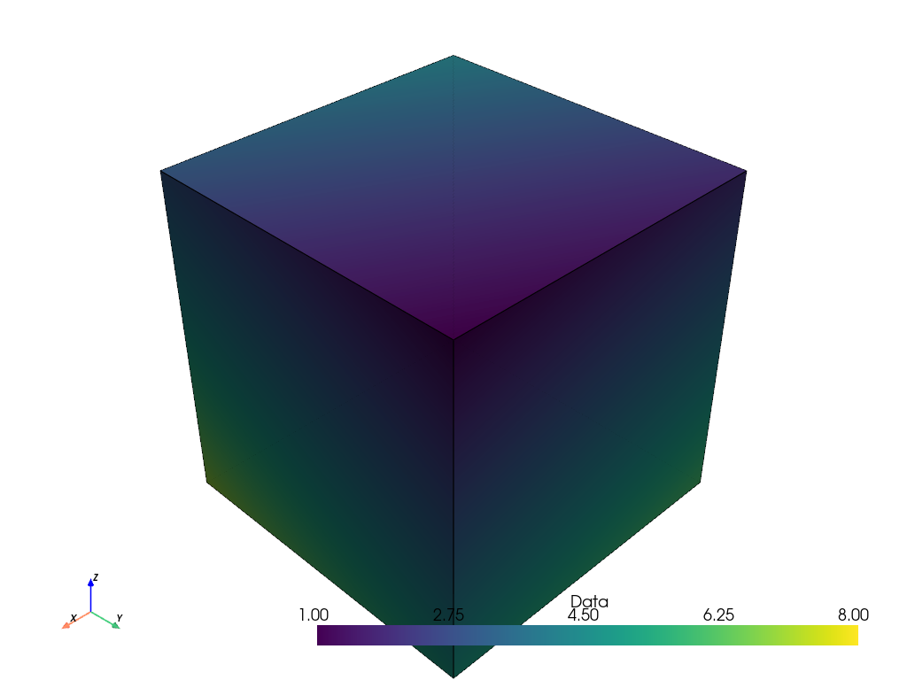
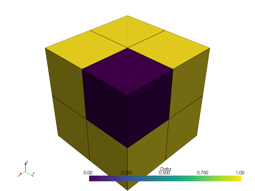
If we plot the volume, it is represented as a single cell with eight points, and the point data is interpolated to color the cell.

points_volume.plot(show_edges=True)

Static Scene

Interactive Scene

However, in many applications (e.g. 3D medical imaging), the scalar data arrays represent discretized samples at the centers of voxels. As such, it may be more appropriate to represent the data as eight voxel cells instead of eight points. We can use points_to_cells() to generate a cell-based representation.

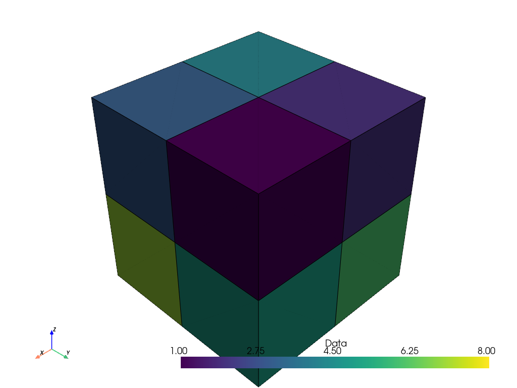
cells_volume = points_volume.points_to_cells()

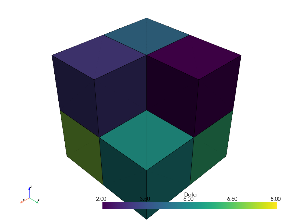
Now, when we plot the volume, we have a more appropriate representation with eight voxel cells and the scalar data is no longer interpolated.

cells_volume.plot(show_edges=True)

Static Scene

Interactive Scene

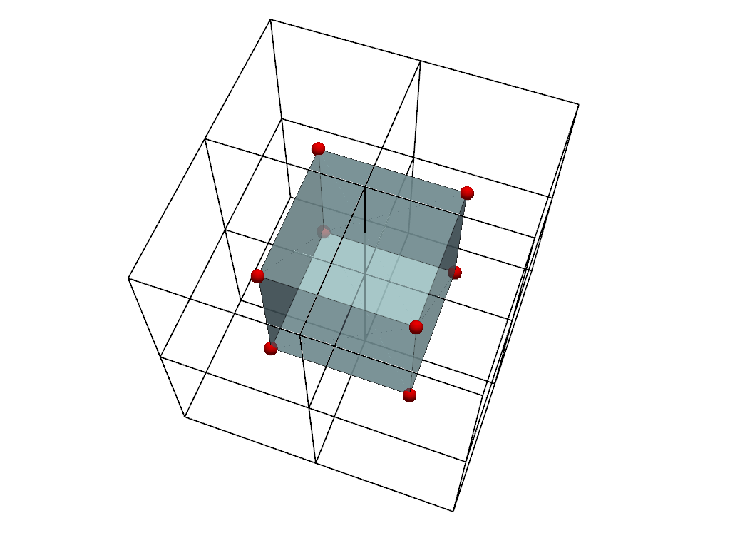
Let’s plot the two representations together for comparison.

For visualization, we color the points volume (inner mesh) and only show the edges of the cells volume (outer mesh). We also plot the cell centers in red. Note how the centers of the image of the cells correspond to the points of the points image.

cell_centers = cells_volume.cell_centers()
cell_edges = cells_volume.extract_all_edges()

plot = pv.Plotter()
plot.add_mesh(points_volume, color=True, show_edges=True, opacity=0.7)
plot.add_mesh(cell_edges, color='black', line_width=2)
plot.add_points(
    cell_centers,
    render_points_as_spheres=True,
    color='red',
    point_size=20,
)
plot.camera.azimuth = -25
plot.camera.elevation = 25
plot.show()

Static Scene

Interactive Scene

As long as only one kind of scalar data is used (i.e. either point or cell data, but not both), it is possible to move between representations without loss of data.

array_before = points_volume.active_scalars
array_after = points_volume.points_to_cells().cells_to_points().active_scalars
np.array_equal(array_before, array_after)

True

Point Filters with Image Data

Use a point representation of the image when working with point-based filters such as image_threshold(). If the image only has cell data, use cells_to_points() re-mesh the input first. Here, we reuse the point-based image defined earlier.

For context, we first show the input data array.

points_volume.point_data['Data']

pyvista_ndarray([8, 7, 6, 5, 4, 3, 2, 1])

Now apply the filter and print the result.

points_ithresh = points_volume.image_threshold(2)
points_ithresh.point_data['Data']

pyvista_ndarray([1, 1, 1, 1, 1, 1, 1, 0])

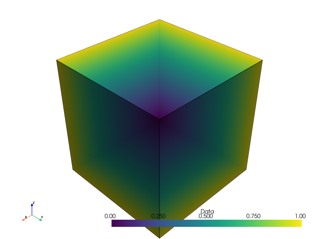
The filter returns binary point data as expected. Values equal to or greater or than the threshold of 2 are ones and less than the threshold are zeros.

However, in plotting it, the point values are linearly interpolated. For visualizing binary data, this interpolation is not desirable.

points_ithresh.plot(show_edges=True)

Static Scene

Interactive Scene

To better visualize the result, convert the image of the point returned by the filter to a cell representation with points_to_cells() before plotting.

points_ithresh_as_cells = points_ithresh.points_to_cells()
points_ithresh_as_cells.plot(show_edges=True)

Static Scene

Interactive Scene

The binary data is now correctly visualized as binary data.

Cell Filters with Image Data

Use a cell representation of the image when working with cell-based filters such as threshold(). If the image only has point data, use points_to_cells() to re-mesh the input first. Here, we reuse the cell-based image created earlier.

For context, we first show the input data array.

cells_volume.cell_data['Data']

pyvista_ndarray([8, 7, 6, 5, 4, 3, 2, 1])

Now apply the filter and print the result.

cells_thresh = cells_volume.threshold(2)
cells_thresh.cell_data['Data']

pyvista_ndarray([8, 7, 6, 5, 4, 3, 2])

When the input is cell data, this filter returns seven discrete values greater than or equal to the threshold value of 2 as expected.

If we plot the result, the cells also produce the correct visualization.

cells_thresh.plot(show_edges=True)

Static Scene

Interactive Scene

However, if we apply the same filter to a point-based representation of the image, the filter does not produce the desired result.

points_thresh = points_volume.threshold(2)
points_thresh.point_data['Data']

pyvista_ndarray([8, 7, 6, 5, 4, 3, 2, 1])

In this case, since the image of the point only has a single cell, the filter has no effect on the data array’s values. The thresholded values are the same as the input values.

Plotting the result confirms this. The plot is identical to the initial plot of the point-based image shown at the beginning of this example.

points_thresh.plot(show_edges=True)

Static Scene

Interactive Scene

Representations of 2D Images

The filters points_to_cells() and cells_to_points() can similarly be used with 2D images.

For this example, we create a 4x4 2D grayscale image with 16 points to represent 16 pixels.

data_array = np.linspace(0, 255, 16, dtype=np.uint8)[::-1]
points_image = pv.ImageData(dimensions=(4, 4, 1))
points_image.point_data['Data'] = data_array

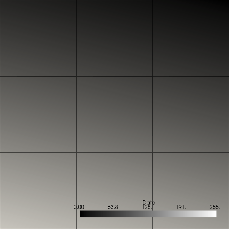
Plot the image. As before, the plot does not appear correct since the point data is interpolated, and nine cells are shown rather than the desired 16 (one for each pixel).

plot_kwargs = dict(
    cpos='xy',
    zoom='tight',
    show_axes=False,
    cmap='gray',
    clim=[0, 255],
    show_edges=True,
)
points_image.plot(**plot_kwargs)

Static Scene

Interactive Scene

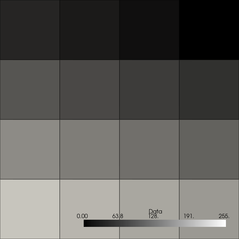
To visualize the image correctly, we first use points_to_cells() to get a cell-based representation of the image and plot the result. The plot now correctly shows 16-pixel cells with discrete values.

cells_image = points_image.points_to_cells()
cells_image.plot(**plot_kwargs)

Static Scene

Interactive Scene

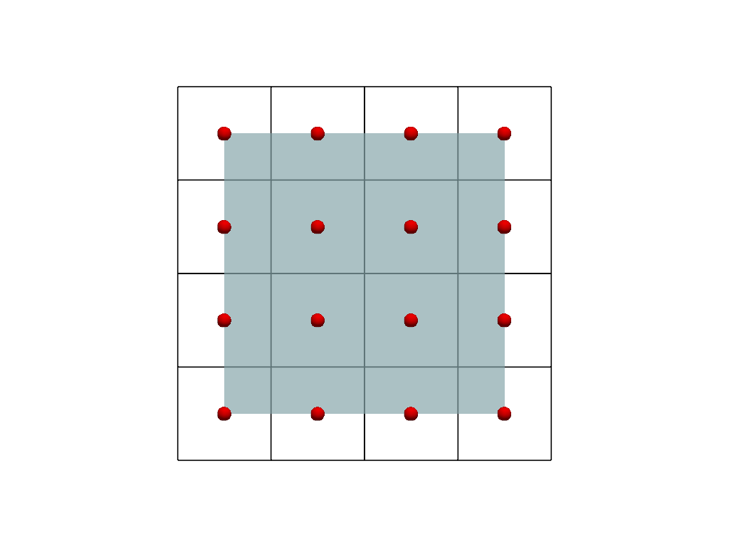
Let’s plot the two representations together for comparison.

For visualization, we color the points image (inner mesh) and show the cells image (outer mesh) as a wireframe. We also plot the cell centers in red. Note how the centers of the image of the cells correspond to the points of the points image.

cell_centers = cells_image.cell_centers()

plot = pv.Plotter()
plot.add_mesh(points_image, color=True, opacity=0.7)
plot.add_mesh(cells_image, style='wireframe', color='black', line_width=2)
plot.add_points(
    cell_centers,
    render_points_as_spheres=True,
    color='red',
    point_size=20,
)
plot.view_xy()
plot.show()

Static Scene

Interactive Scene