Note
Go to the end to download the full example code.
Connectivity#
This example highlights some applications of the
connectivity() filter.
Remove Noisy Isosurfaces#
Use connectivity to remove noisy isosurfaces.
This section is similar to this VTK example.
import numpy as np
import pyvista as pv
from pyvista import examples
Load a dataset with noisy isosurfaces.
pine_roots = examples.download_pine_roots()

# Plot the raw data
cpos = pv.CameraPosition(
    position=(40.6018, -280.533, 47.0172),
    focal_point=(40.6018, 37.2813, 50.1953),
    viewup=(0.0, 0.0, 1.0),
)
pl = pv.Plotter()
pl.add_mesh(pine_roots, color='#965434')
pl.add_mesh(pine_roots.outline())
pl.show(cpos=cpos)
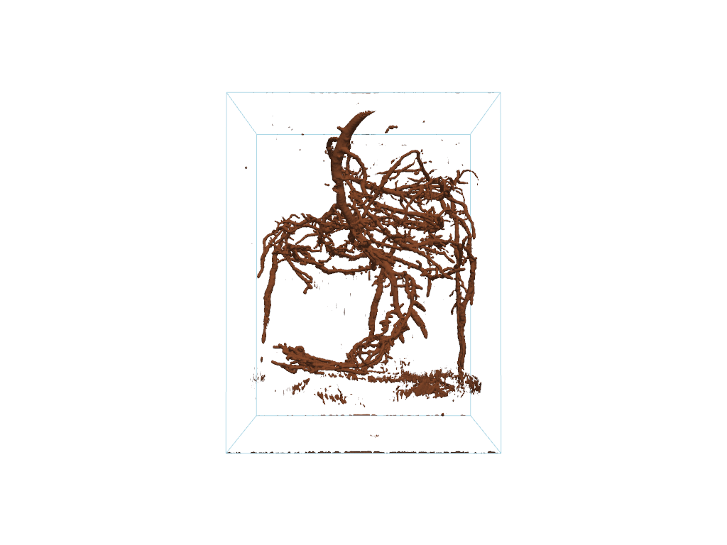
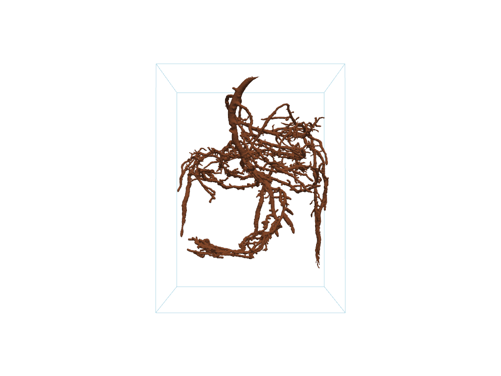
The plotted mesh is very noisy. We can extract the largest connected
isosurface using the 'largest' extraction_mode of the
connectivity() filter. Equivalently,
extract_largest() may also be used.
# Grab the largest connected volume present
largest = pine_roots.connectivity('largest')
# or: largest = mesh.extract_largest()

pl = pv.Plotter()
pl.add_mesh(largest, color='#965434')
pl.add_mesh(pine_roots.outline())
pl.camera_position = cpos
pl.show()
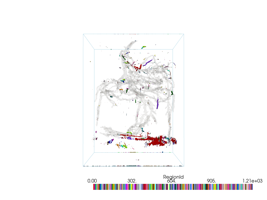
Extract Small Regions#
Use connectivity to extract the smaller ‘noisy’ regions that were removed in the remove noisy isosurfaces example above.
First, get a list of all region ids.
all_regions = pine_roots.connectivity('all')
region_ids = np.unique(all_regions['RegionId'])
Since the region IDs are sorted in descending order (by cell count),
we can extract all regions except for the largest one using the
'specified' extraction_mode of the connectivity()
filter.
noise_region_ids = region_ids[1::]  # All region ids except '0'
noise = pine_roots.connectivity('specified', noise_region_ids)
Plot the noisy regions using color_labels().
For context, also plot the largest region.
pl = pv.Plotter()
pl.add_mesh(noise.color_labels())
pl.add_mesh(largest, color='lightgray', opacity=0.1)
pl.add_mesh(pine_roots.outline())
pl.camera_position = cpos
pl.show()
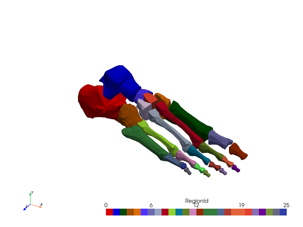
Label Disconnected Regions#
Use connectivity to label all disconnected regions.
This section is similar to this VTK example.
First, load a dataset with disconnected regions.
mesh = examples.download_foot_bones()
Extract all regions.
conn = mesh.connectivity('all')
Plot the labeled regions using color_labels().
colored = conn.color_labels()
cpos = pv.CameraPosition(
    position=(10.5, 12.2, 18.3), focal_point=(0.0, 0.0, 0.0), viewup=(0.0, 1.0, 0.0)
)
colored.plot(cpos=cpos)
Extract Regions From Seed Points#
Use connectivity to extract regions of interest using scalar data and seed points.
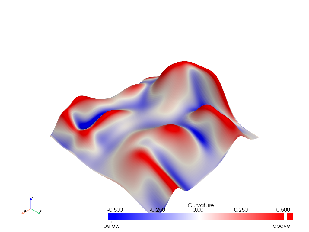
First, create a dataset with salient features. Here, we create hills and use curvature to define its peaks and valleys.
mesh = pv.ParametricRandomHills()
mesh['Curvature'] = mesh.curvature()
Visualize the peaks and valleys. Peaks have large positive curvature (i.e. are convex). Valleys have large negative curvature (i.e. are concave). Flat regions have curvature close to zero.
mesh.plot(
    clim=[-0.5, 0.5],
    cmap='bwr',
    below_color='blue',
    above_color='red',
)
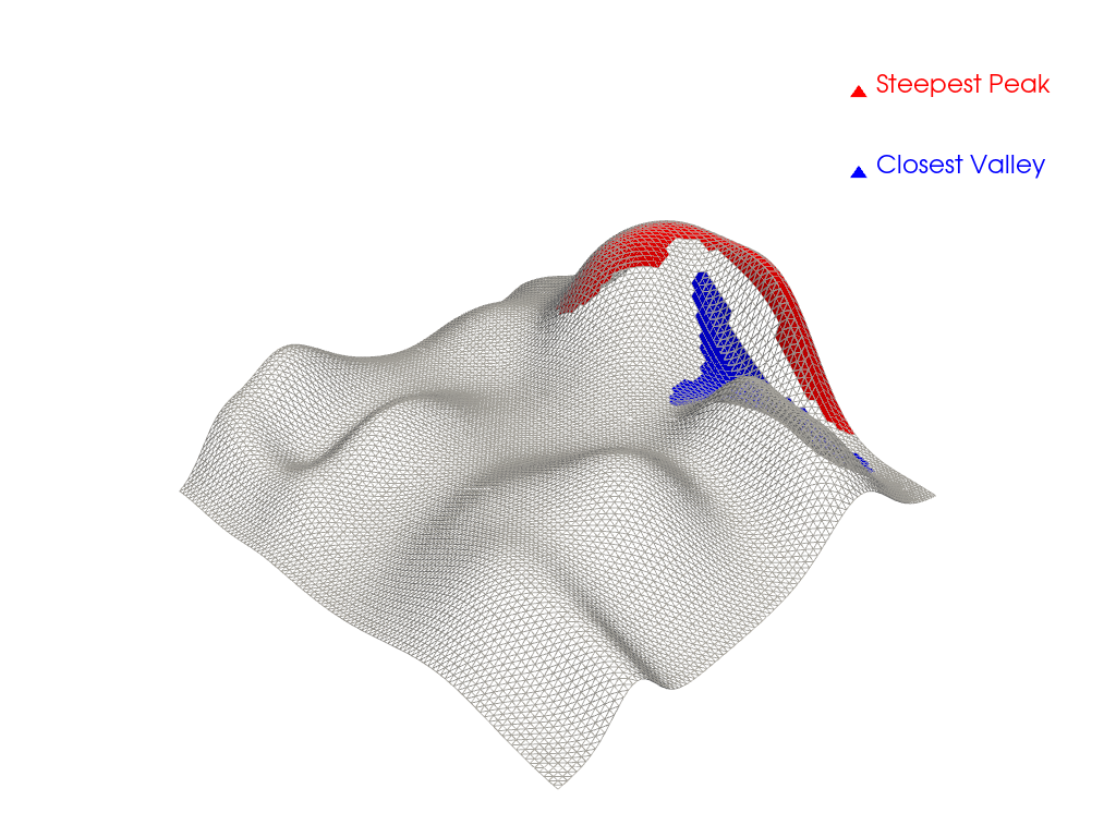
Extract a region of interest using the
'point_seed' extraction_mode of the connectivity()
filter. Let’s extract the steepest peak using a seed point where the
curvature is maximized.
# Get seed point
peak_point_id = np.argmax(mesh['Curvature'])

# Define a scalar range of the region to extract
data_min, data_max = mesh.get_data_range()
peak_range = [0.2, data_max]  # Peak if curvature > 0.2

peak_mesh = mesh.connectivity('point_seed', peak_point_id, scalar_range=peak_range)
Let’s also extract the closest valley to the steepest peak using the
'closest' extraction_mode of the connectivity()
filter.
valley_range = [data_min, -0.2]  # Valley if curvature < -0.2
peak_point = mesh.points[peak_point_id]
valley_mesh = mesh.connectivity('closest', peak_point, scalar_range=valley_range)
Plot extracted regions.
pl = pv.Plotter()
_ = pl.add_mesh(mesh, style='wireframe', color='lightgray')
_ = pl.add_mesh(peak_mesh, color='red', label='Steepest Peak')
_ = pl.add_mesh(valley_mesh, color='blue', label='Closest Valley')
_ = pl.add_legend()
pl.show()
Total running time of the script: (0 minutes 5.179 seconds)