Scaled Gaussian Points

This example demonstrates how to plot spheres using the 'points_gaussian' style and scale them by a dynamic radius.

from __future__ import annotations

import numpy as np

import pyvista as pv

First, generate the sphere positions and radii randomly on the edge of a torus.

# Seed the rng for reproducibility
rng = np.random.default_rng(seed=0)

N_SPHERES = 10_000
theta = rng.uniform(0, 2 * np.pi, N_SPHERES)
phi = rng.uniform(0, 2 * np.pi, N_SPHERES)
torus_radius = 1
tube_radius = 0.3
radius = torus_radius + tube_radius * np.cos(phi)
rad = rng.random(N_SPHERES) * 0.01

pos = np.zeros((N_SPHERES, 3))
pos[:, 0] = radius * np.cos(theta)
pos[:, 1] = radius * np.sin(theta)
pos[:, 2] = tube_radius * np.sin(phi)

Next, create a PolyData object and add the sphere positions and radii as data arrays.

pdata = pv.PolyData(pos)
pdata['radius'] = rad

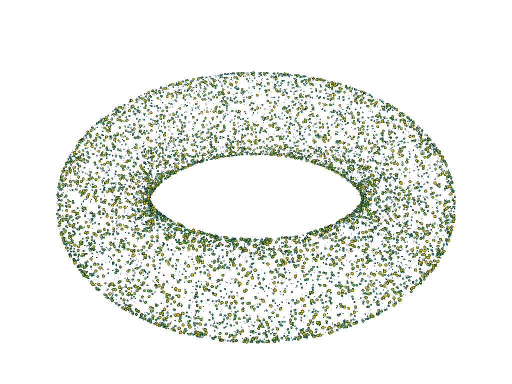
Finally, plot the spheres using the points_gaussian style and scale them by radius.

pl = pv.Plotter()
actor = pl.add_mesh(
    pdata,
    style='points_gaussian',
    emissive=False,
    render_points_as_spheres=True,
    show_scalar_bar=False,
)
actor.mapper.scale_array = 'radius'
pl.camera.zoom(1.5)
pl.show()

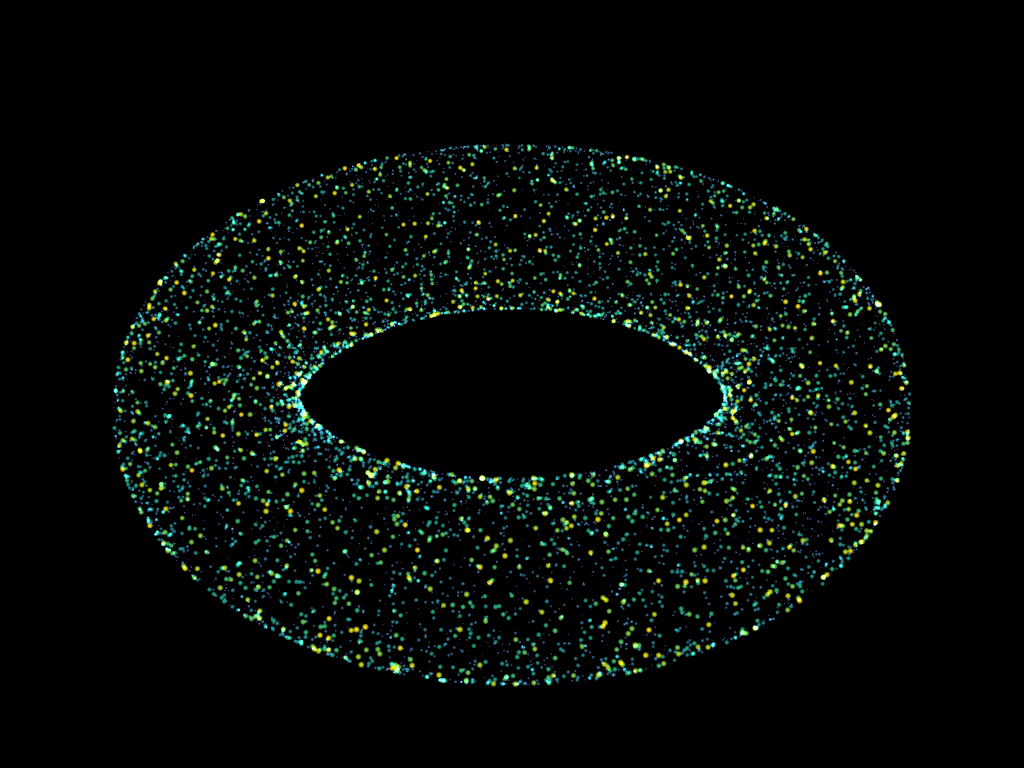
Show the same plot with emissive=True.

pl = pv.Plotter()
pl.background_color = 'k'
actor = pl.add_mesh(
    pdata,
    style='points_gaussian',
    emissive=True,
    render_points_as_spheres=True,
    show_scalar_bar=False,
)
actor.mapper.scale_array = 'radius'
pl.camera.zoom(1.5)
pl.show()