Volume Rendering

Volume render uniform mesh types like pyvista.ImageData or 3D NumPy arrays.

This also explores how to extract a volume of interest (VOI) from a pyvista.ImageData using the pyvista.ImageDataFilters.extract_subset() filter.

from __future__ import annotations

import numpy as np

import pyvista as pv
from pyvista import examples


# Download a volumetric dataset
vol = examples.download_knee_full()
vol

Header	Data Arrays
ImageData Information N Cells 10225800 N Points 10368384 X Bounds 0.000e+00, 1.497e+02 Y Bounds 0.000e+00, 1.786e+02 Z Bounds 0.000e+00, 2.000e+02 Dimensions 208, 248, 201 Spacing 7.230e-01, 7.230e-01, 1.000e+00 N Arrays 1	Name Field Type N Comp Min Max SLCImage Points uint8 1 0.000e+00 1.740e+02

Simple Volume Render

# A nice camera position
cpos = [(-381.74, -46.02, 216.54), (74.8305, 89.2905, 100.0), (0.23, 0.072, 0.97)]

vol.plot(volume=True, cmap='bone', cpos=cpos)

Opacity Mappings

Or use the pyvista.Plotter.add_volume() method like below. Note that here we use a non-default opacity mapping to a sigmoid:

pl = pv.Plotter()
pl.add_volume(vol, cmap='bone', opacity='sigmoid')
pl.camera_position = cpos
pl.show()

You can also use a custom opacity mapping

opacity = [0, 0, 0, 0.1, 0.3, 0.6, 1]

pl = pv.Plotter()
pl.add_volume(vol, cmap='viridis', opacity=opacity)
pl.camera_position = cpos
pl.show()

We can also use a shading technique when volume rendering with the shade option

pl = pv.Plotter(shape=(1, 2))
pl.add_volume(vol, cmap='viridis', opacity=opacity, shade=False)
pl.add_text('No shading')
pl.camera_position = cpos
pl.subplot(0, 1)
pl.add_volume(vol, cmap='viridis', opacity=opacity, shade=True)
pl.add_text('Shading')
pl.link_views()
pl.show()

Cool Volume Examples

Here are a few more cool volume rendering examples.

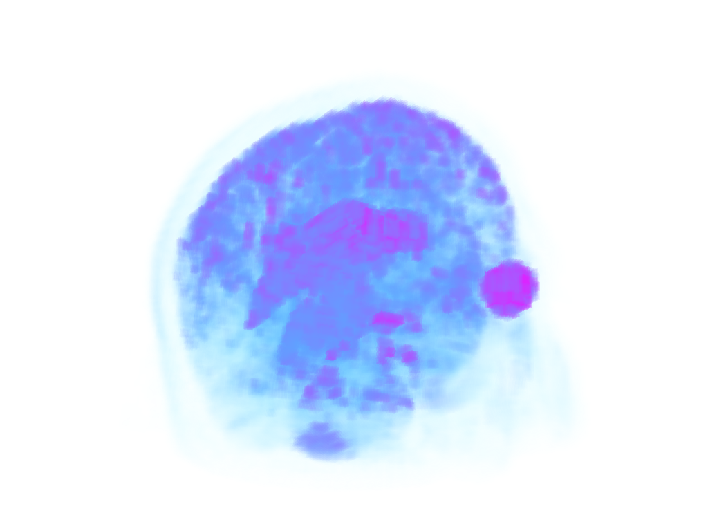
Head Dataset

head = examples.download_head()

pl = pv.Plotter()
pl.add_volume(head, cmap='cool', opacity='sigmoid_6', show_scalar_bar=False)
pl.camera_position = [(-228.0, -418.0, -158.0), (94.0, 122.0, 82.0), (-0.2, -0.3, 0.9)]
pl.camera.zoom(1.5)
pl.show()

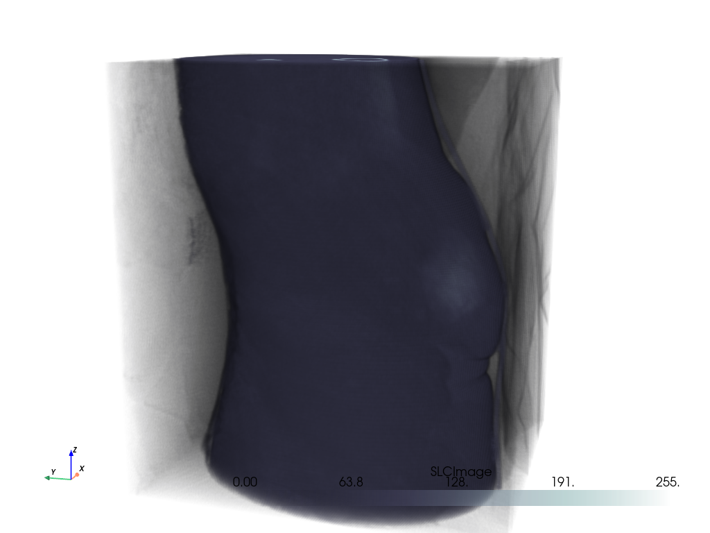
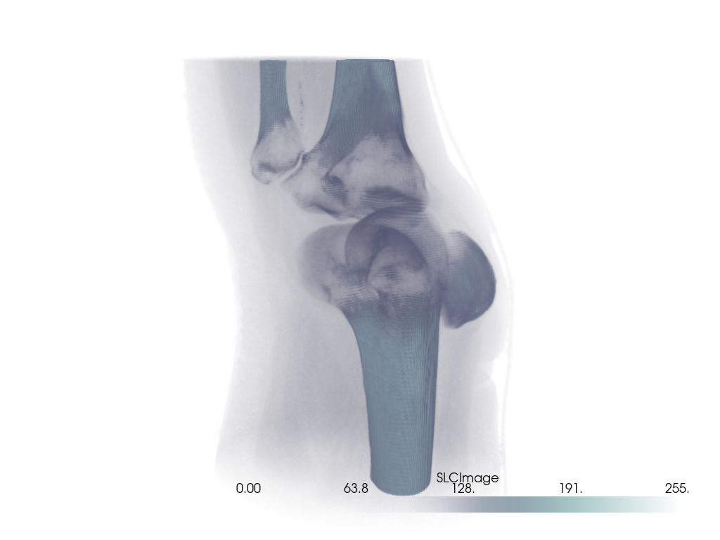
Bolt-Nut MultiBlock Dataset

Note

See how we set interpolation to 'linear' here to smooth out scalars of each individual cell to make a more appealing plot. Two actor are returned by add_volume because bolt_nut is a pyvista.MultiBlock dataset.

bolt_nut = examples.download_bolt_nut()

pl = pv.Plotter()
actors = pl.add_volume(bolt_nut, cmap='coolwarm', opacity='sigmoid_5', show_scalar_bar=False)
actors[0].prop.interpolation_type = 'linear'
actors[1].prop.interpolation_type = 'linear'
pl.camera_position = [(127.4, -68.3, 88.2), (30.3, 54.3, 26.0), (-0.25, 0.28, 0.93)]
cpos = pl.show(return_cpos=True)

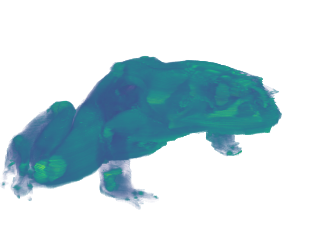
Frog Dataset

frog = examples.download_frog()

pl = pv.Plotter()
pl.add_volume(frog, cmap='viridis', opacity='sigmoid_6', show_scalar_bar=False)
pl.camera_position = [(929.0, 1067.0, -278.9), (249.5, 234.5, 101.25), (-0.2048, -0.2632, -0.9427)]
pl.camera.zoom(1.5)
pl.show()

Extracting a VOI

Use the pyvista.ImageDataFilters.extract_subset() filter to extract a volume of interest/subset volume to volume render. This is ideal when dealing with particularly large volumes and you want to volume render only a specific region.

# Load a particularly large volume
large_vol = examples.download_damavand_volcano()
large_vol

Header	Data Arrays
ImageData Information N Cells 11003760 N Points 11156040 X Bounds 4.130e+05, 6.920e+05 Y Bounds 3.864e+06, 4.096e+06 Z Bounds -5.479e+04, 5.302e+03 Dimensions 280, 233, 171 Spacing 1.000e+03, 1.000e+03, 3.535e+02 N Arrays 1	Name Field Type N Comp Min Max data Points float32 1 9.782e-15 1.000e+02

opacity = [0, 0.75, 0, 0.75, 1.0]
clim = [0, 100]

pl = pv.Plotter()
pl.add_volume(
    large_vol,
    cmap='magma',
    clim=clim,
    opacity=opacity,
    opacity_unit_distance=6000,
)
pl.show()

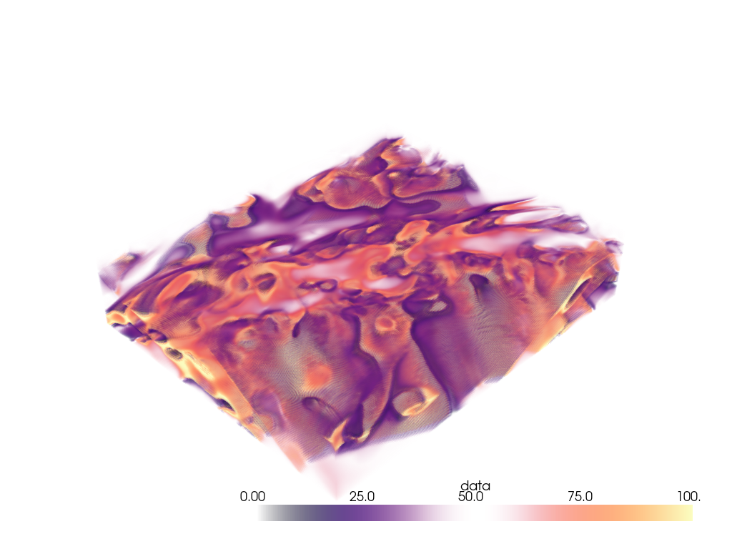
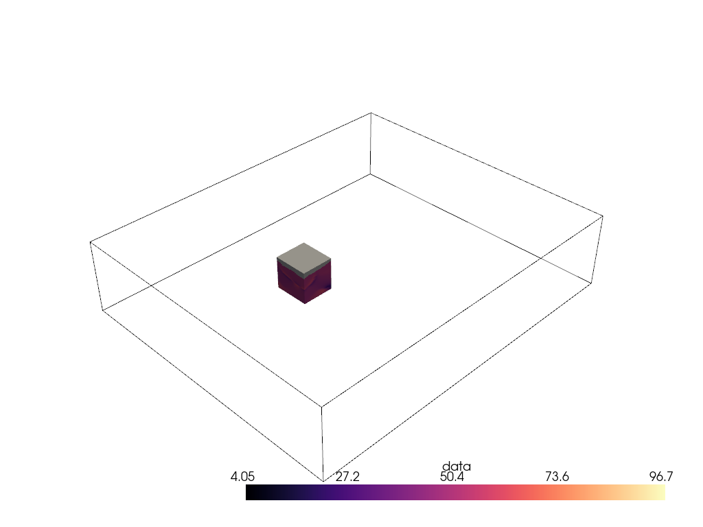
Woah, that’s a big volume. We probably don’t want to volume render the whole thing. So let’s extract a region of interest under the volcano.

The region we will extract will be between nodes 175 and 200 on the x-axis, between nodes 105 and 132 on the y-axis, and between nodes 98 and 170 on the z-axis.

voi = large_vol.extract_subset([175, 200, 105, 132, 98, 170])

pl = pv.Plotter()
pl.add_mesh(large_vol.outline(), color='k')
pl.add_mesh(voi, cmap='magma')
pl.show()

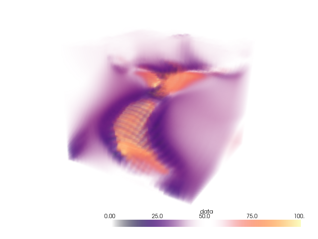
Ah, much better. Let’s now volume render that region of interest.

pl = pv.Plotter()
pl.add_volume(voi, cmap='magma', clim=clim, opacity=opacity, opacity_unit_distance=2000)
pl.camera_position = [
    (531554.5542909054, 3944331.800171338, 26563.04809259223),
    (599088.1433822059, 3982089.287834022, -11965.14728669936),
    (0.3738545892415734, 0.244312810377319, 0.8947312427698892),
]
pl.show()

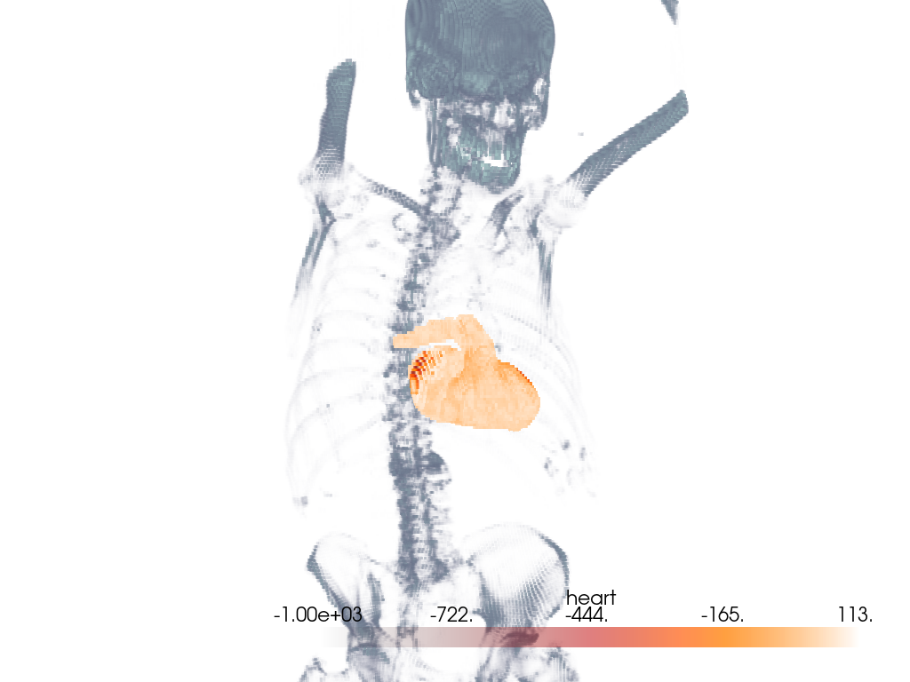
Volume With Segmentation Mask

Visualize a medical image with a corresponding binary segmentation mask.

For this example, we use download_whole_body_ct_male() though download_whole_body_ct_female(), or any other dataset with a corresponding label or mask may be used.

Load the dataset and get the ct image and a mask image. Here, a mask of the heart is used.

dataset = examples.download_whole_body_ct_male()
ct_image = dataset['ct']
heart_mask = dataset['segmentations']['heart']

Use the segmentation mask to isolate the heart in the CT image.

Initialize a new array and image with CT background values. Here, we set the scalar values to -1000 which typically corresponds to air (low density).

heart_array = np.full_like(ct_image.active_scalars, -1000)

Extract the intensities for the heart segment. We use heart mask’s array to mask the CT image to only extract the intensities of interest.

ct_image_array = ct_image.active_scalars
heart_mask_array = heart_mask.active_scalars
heart_array[heart_mask_array == True] = ct_image_array[heart_mask_array == True]  # noqa: E712

Add the masked array to the CT image as a new set of scalar values.

ct_image['heart'] = heart_array

Create the plot.

For the CT image, the opacity is set to a sigmoid function to show the subject’s skeleton. Since different images have different intensity distributions, you may need to experiment with different sigmoid functions. See add_volume() for details.

pl = pv.Plotter()

# Add the CT image.
pl.add_volume(
    ct_image,
    scalars='NIFTI',
    cmap='bone',
    opacity='sigmoid_15',
    show_scalar_bar=False,
)

# Add masked CT image of the heart and use a contrasting color map.
_ = pl.add_volume(
    ct_image,
    scalars='heart',
    cmap='gist_heat',
    opacity='linear',
    opacity_unit_distance=np.mean(ct_image.spacing),
)

# Orient the camera to provide a latero-anterior view.
pl.view_yz()
pl.camera.azimuth = 70
pl.camera.up = (0, 0, 1)
pl.camera.zoom(1.5)
pl.show()

Tags: medical plot