pyvista.PolyDataFilters.ray_trace

PolyDataFilters.ray_trace(

origin,

end_point,

first_point: bool = False,

plot: bool = False,

off_screen=None,

)

Perform a single ray trace calculation.

This requires a mesh and a line segment defined by an origin and end_point.

Warning

This filter uses the mesh’s obbTree property internally to compute the intersection. Since the obb tree is cached, the intersection may not be valid if the mesh’s geometry is modified in between filter calls.

Parameters:

originsequence[float]

Start of the line segment.

end_pointsequence[float]

End of the line segment.

first_pointbool, default: False

Returns intersection of first point only.

plotbool, default: False

Whether to plot the ray trace results.

off_screenbool, optional

Plots off screen when plot=True. Used for unit testing.

Returns:

intersection_pointsnumpy.ndarray

Location of the intersection points. Empty array if no intersections.

intersection_cellsnumpy.ndarray

Indices of the intersection cells. Empty array if no intersections.

See also

Visualize the Moeller-Trumbore Algorithm

Example of ray-tracing using the Moeller-Trumbore intersection algorithm.

Examples

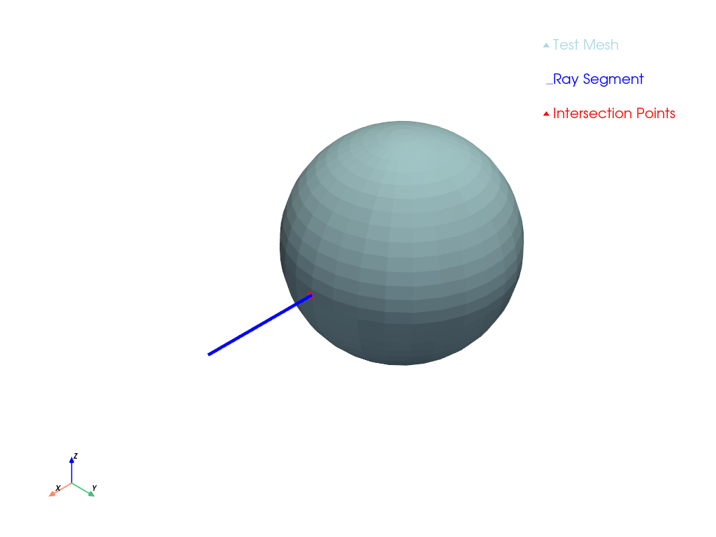
Compute the intersection between a ray from the origin to [1, 0, 0] and a sphere with radius 0.5 centered at the origin.

>>> import pyvista as pv
>>> sphere = pv.Sphere()
>>> point, cell = sphere.ray_trace([0, 0, 0], [1, 0, 0], first_point=True)
>>> f'Intersected at {point[0]:.3f} {point[1]:.3f} {point[2]:.3f}'
'Intersected at 0.499 0.000 0.000'

Show a plot of the ray trace.

>>> point, cell = sphere.ray_trace([0, 0, 0], [1, 0, 0], plot=True)

See Ray Tracing for more examples using this filter.

Static Scene

Interactive Scene