Point Sets#

PyVista point sets are datasets with explicit geometry where the point and cell topology are specified and not inferred. PyVista point sets are modeled after the same data model as VTK’s point sets while being designed to make creation, array access, and plotting more straightforward than their VTK counterparts.

The pyvista.UnstructuredGrid class is used for arbitrary combinations of all possible cell types:

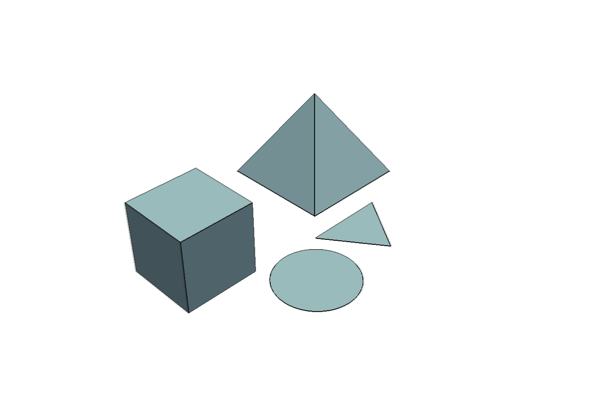
The pyvista.PolyData is used for datasets consisting of surface geometry (for example vertices, lines, and polygons):

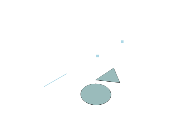
The pyvista.StructuredGrid is used for topologically regular arrays of data:

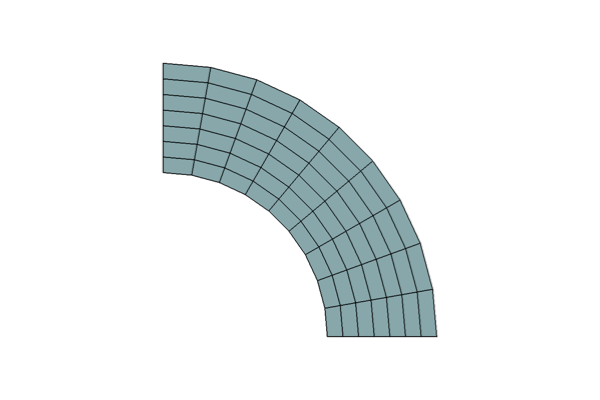
The pyvista.PointSet (as of vtk==9.1.0) is a concrete class for storing a set of points.

Class Descriptions

The following table describes PyVista’s point set classes. These classes inherit all methods from their corresponding VTK vtkPointSet, vtkPolyData, vtkUnstructuredGrid, vtkStructuredGrid, and vtkExplicitStructuredGrid superclasses.

`pyvista.PointSet`(args, *kwargs)	Concrete class for storing a set of points.
`pyvista.PolyData`(args, *kwargs)	Dataset consisting of surface geometry (e.g. vertices, lines, and polygons).
`pyvista.UnstructuredGrid`(args, *kwargs)	Dataset used for arbitrary combinations of all possible cell types.
`pyvista.StructuredGrid`(args, *kwargs)	Dataset used for topologically regular arrays of data.
`pyvista.ExplicitStructuredGrid`(args, *kwargs)	Extend the functionality of the `vtk.vtkExplicitStructuredGrid` class.

PolyData Creation#

Empty Object#

A pyvista.PolyData object can be initialized with:

import pyvista
mesh = pyvista.PolyData()

This creates an mesh, which you can then add

Points with points
Vertices with verts
Lines with lines
Faces with faces

Note that unlike pyvista.UnstructuredGrid, you do not specify cell types. All faces are assumed to be polygons, hence the name “Poly” data.

Click on the attributes above to see examples of how to add geometric features to an empty. See Create PolyData for an example on creating a pyvista.PolyData object from NumPy arrays.

Initialize from a File#

Both binary and ASCII .ply, .stl, and .vtk files can be read using PyVista. For example, the PyVista package contains example meshes and these can be loaded with:

import pyvista
from pyvista import examples

# Load mesh
mesh = pyvista.PolyData(examples.planefile)
mesh

PolyData	Information
N Cells	2452
N Points	1335
N Strips	0
X Bounds	1.391e+02, 1.655e+03
Y Bounds	3.209e+01, 1.320e+03
Z Bounds	-1.774e+01, 2.821e+02
N Arrays	0

This mesh can then be written to a .vtk file using:

mesh.save('plane.vtk')

These meshes are identical.

import numpy as np

mesh_from_vtk = pyvista.PolyData('plane.vtk')
print(np.allclose(mesh_from_vtk.points, mesh.points))

Mesh Manipulation and Plotting#

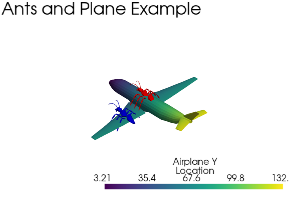
Meshes can be directly manipulated using NumPy or with the built-in translation and rotation routines. This example loads two meshes and moves, scales, copies them, and finally plots them.

To plot more than one mesh a pyvista.Plotter instance must be created to manage the plotting. The following code creates a plotter and plots the meshes with various colors.

import pyvista
from pyvista import examples

# load and shrink airplane
airplane = pyvista.PolyData(examples.planefile)
airplane.points /= 10 # shrink by 10x

# rotate and translate ant so it is on the plane
ant = pyvista.PolyData(examples.antfile)
ant.rotate_x(90, inplace=True)
ant.translate([90, 60, 15], inplace=True)

# Make a copy and add another ant
ant_copy = ant.copy()
ant_copy.translate([30, 0, -10], inplace=True)

# Create plotter object
plotter = pyvista.Plotter()
plotter.add_mesh(ant, 'r')
plotter.add_mesh(ant_copy, 'b')

# Add airplane mesh and make the color equal to the Y position. Add a
# scalar bar associated with this mesh
plane_scalars = airplane.points[:, 1]
plotter.add_mesh(airplane, scalars=plane_scalars,
                 scalar_bar_args={'title': 'Airplane Y\nLocation'})

# Add annotation text
plotter.add_text('Ants and Plane Example')
plotter.show()

Unstructured Grid Creation#

See Creating an Unstructured Grid for an example on how to create an unstructured grid from NumPy arrays.

Create#

An unstructured grid can be initialized with:

import pyvista as pv
grid = pv.UnstructuredGrid()

This creates an empty grid, and is it not useful until points and cells are added to it. Points and cells can be added later with points, cells, and celltypes .

Alternatively, you can add points and cells directly when initializing.

>>> import numpy as np
>>> import pyvista
>>> from pyvista import CellType
>>> cells = np.array([8, 0, 1, 2, 3, 4, 5, 6, 7, 8, 8, 9, 10, 11, 12, 13, 14, 15])
>>> cell_type = np.array([CellType.HEXAHEDRON, CellType.HEXAHEDRON], np.int8)
>>> cell1 = np.array([[0, 0, 0],
...                   [1, 0, 0],
...                   [1, 1, 0],
...                   [0, 1, 0],
...                   [0, 0, 1],
...                   [1, 0, 1],
...                   [1, 1, 1],
...                   [0, 1, 1]], dtype=np.float32)
>>> cell2 = np.array([[0, 0, 2],
...                   [1, 0, 2],
...                   [1, 1, 2],
...                   [0, 1, 2],
...                   [0, 0, 3],
...                   [1, 0, 3],
...                   [1, 1, 3],
...                   [0, 1, 3]], dtype=np.float32)
>>> points = np.vstack((cell1, cell2))
>>> grid = pyvista.UnstructuredGrid(cells, cell_type, points)
>>> grid

UnstructuredGrid	Information
N Cells	2
N Points	16
X Bounds	0.000e+00, 1.000e+00
Y Bounds	0.000e+00, 1.000e+00
Z Bounds	0.000e+00, 3.000e+00
N Arrays	0

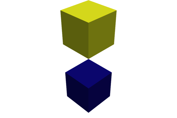
We can plot this with colors with:

>>> grid.plot(scalars=[0, 1], cmap='plasma')

Loading from File#

Unstructured grids can be loaded from a vtk file.

import pyvista as pv
from pyvista import examples

grid = pv.UnstructuredGrid(examples.hexbeamfile)
grid

Header

Data Arrays

UnstructuredGrid	Information
N Cells	40
N Points	99
X Bounds	0.000e+00, 1.000e+00
Y Bounds	0.000e+00, 1.000e+00
Z Bounds	0.000e+00, 5.000e+00
N Arrays	3

Name	Field	Type	N Comp	Min	Max
sample_point_scalars	Points	int64	1	1.000e+00	3.020e+02
VTKorigID	Points	int64	1	0.000e+00	9.800e+01
sample_cell_scalars	Cells	int32	1	1.000e+00	4.000e+01

Structured Grid Creation#

Empty Object#

A structured grid can be initialized with:

import pyvista as pv
grid = pv.StructuredGrid()

Creating from NumPy Arrays#

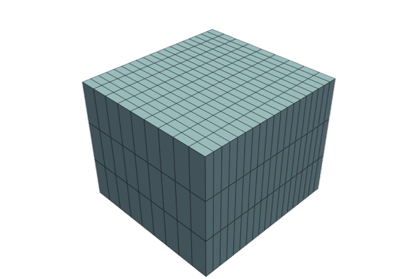
A structured grid can be created directly from numpy arrays. This is useful when creating a grid from scratch or copying it from another format.

Also see Creating a Structured Surface for an example on creating a structured grid from NumPy arrays.

import pyvista as pv
import numpy as np

x = np.arange(-10, 10, 1, dtype=np.float32)
y = np.arange(-10, 10, 2, dtype=np.float32)
z = np.arange(-10, 10, 5, dtype=np.float32)
x, y, z = np.meshgrid(x, y, z, indexing='ij')

# create the unstructured grid directly from the numpy arrays and plot
grid = pv.StructuredGrid(x, y, z)
grid.plot(show_edges=True)

Loading from File#

Structured grids can be loaded from a vtk file.

grid = pv.StructuredGrid(filename)

Plotting Grids#

This example shows how you can load an unstructured grid from a vtk file and create a plot and GIF movie by updating the plotting object.

# Load module and example file
import pyvista as pv
from pyvista import examples
import numpy as np

# Load example beam grid
grid = pv.UnstructuredGrid(examples.hexbeamfile)

# Create fictitious displacements as a function of Z location
d = np.zeros_like(grid.points)
d[:, 1] = grid.points[:, 2]**3/250

# Displace original grid
grid.points += d

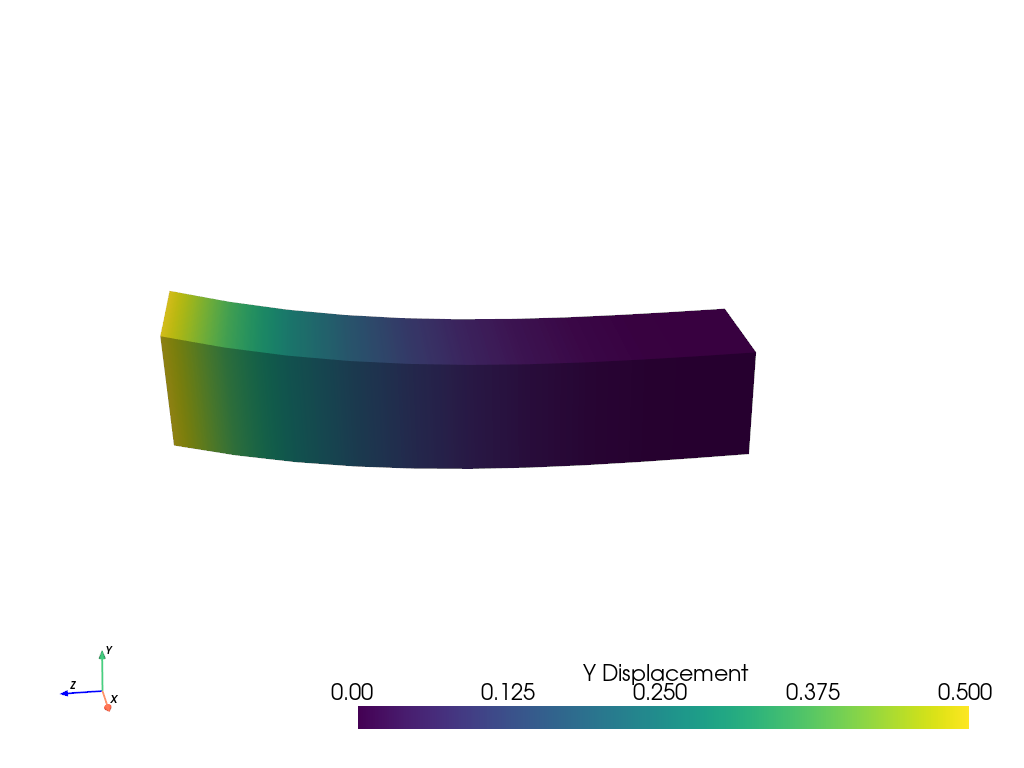
A simple plot can be created by using:

# Camera position.
# it's hard-coded in this example
cpos = [(11.9151, 6.1139, 3.61249),
        (0.0, 0.375, 2.0),
        (-0.4254, 0.9024, -0.0678)]

grid.plot(scalars=d[:, 1], scalar_bar_args={'title': 'Y Displacement'}, cpos=cpos)

Static Scene

Interactive Scene

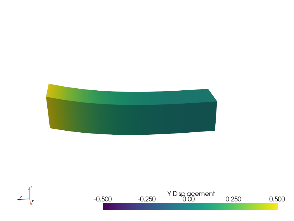
A more complex plot can be created using:

# plot this displaced beam
plotter = pv.Plotter()
plotter.add_mesh(grid, scalars=d[:, 1],
                 scalar_bar_args={'title': 'Y Displacement'},
                 rng=[-d.max(), d.max()])
plotter.add_axes()
plotter.camera_position = cpos
plotter.show()

Static Scene

Interactive Scene

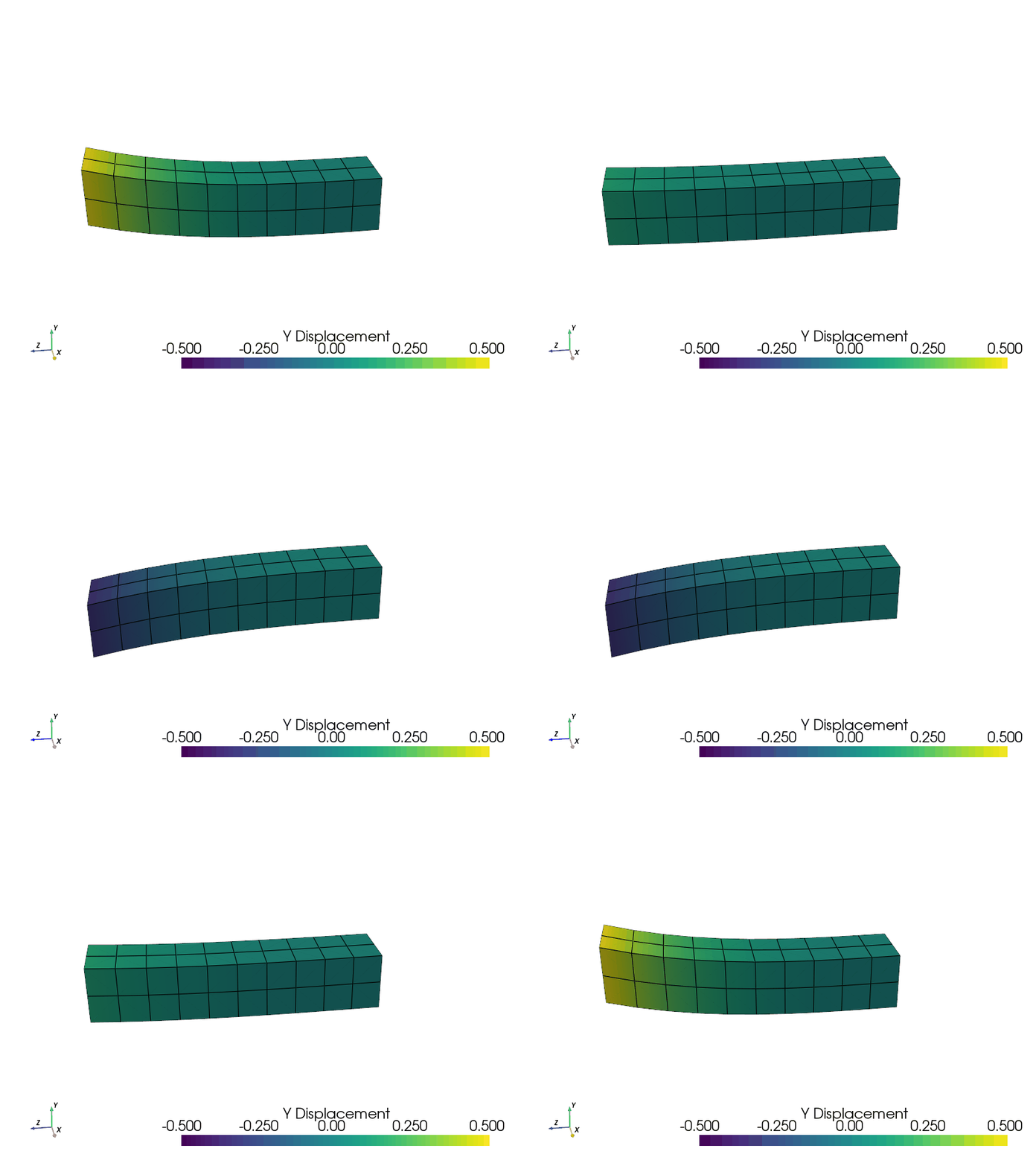
You can animate the motion of the beam by updating the positions and scalars of the grid copied to the plotting object. Here is a full example:

# Load module and example file
import pyvista as pv
from pyvista import examples
import numpy as np

# Load example beam grid
grid = pv.UnstructuredGrid(examples.hexbeamfile)

# Create fictitious displacements as a function of Z location
d = np.zeros_like(grid.points)
d[:, 1] = grid.points[:, 2]**3/250
grid['Y Displacement'] = d[:, 1]

# use hardcoded camera position
cpos = [(11.915, 6.114, 3.612),
        (0.0, 0.375, 2.0),
        (-0.425, 0.902, -0.0679)]

plotter = pv.Plotter(window_size=(800, 600))
plotter.add_mesh(grid, scalars='Y Displacement',
                 show_edges=True, rng=[-d.max(), d.max()],
                 interpolate_before_map=True)
plotter.add_axes()
plotter.camera_position = cpos

# open movie file. A mp4 file can be written instead. Requires ``moviepy``
plotter.open_gif('beam.gif')  # or beam.mp4

# Modify position of the beam cyclically
pts = grid.points.copy()  # unmodified points
for phase in np.linspace(0, 2*np.pi, 20):
    grid.points = pts + d * np.cos(phase)
    grid['Y Displacement'] = d[:, 1] * np.cos(phase)
    plotter.write_frame()

# close the plotter when complete
plotter.close()

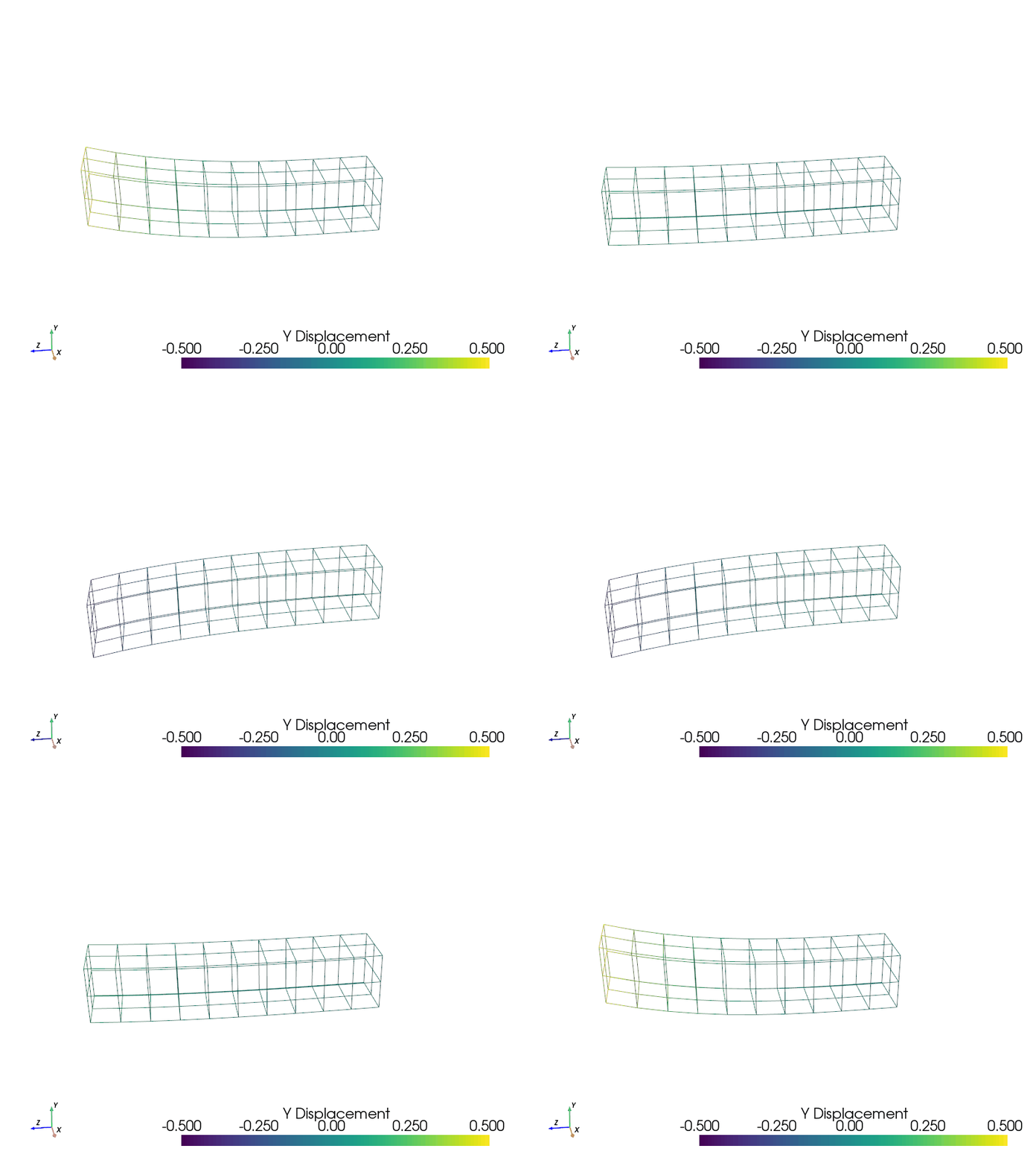
You can also render the beam as a wire-frame object:

# Animate plot as a wire-frame
plotter = pv.Plotter(window_size=(800, 600))
plotter.add_mesh(grid, scalars='Y Displacement',
                 show_edges=True,
                 rng=[-d.max(), d.max()], interpolate_before_map=True,
                 style='wireframe')
plotter.add_axes()
plotter.camera_position = cpos

plotter.open_gif('beam_wireframe.gif')
for phase in np.linspace(0, 2*np.pi, 20):
    grid.points = pts + d * np.cos(phase)
    grid['Y Displacement'] = d[:, 1] * np.cos(phase)
    plotter.write_frame()

# close the plotter when complete
plotter.close()

Adding Labels to a Plot#

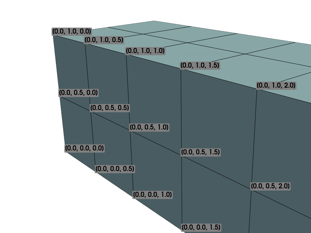
Labels can be added to a plot using add_point_labels() within the Plotter. The following example loads the included example beam, generates a plotting class, and sub-selects points along the y-z plane and labels their coordinates. add_point_labels() requires that the number of labels matches the number of points, and that labels is a list containing one entry per point. The code automatically converts each item in the list to a string.

# Load module and example file
import pyvista as pv
from pyvista import examples

# Load example beam file
grid = pv.UnstructuredGrid(examples.hexbeamfile)

# Create plotting class and add the unstructured grid
plotter = pv.Plotter()
plotter.add_mesh(grid, show_edges=True, color='lightblue')

# Add labels to points on the yz plane (where x == 0)
points = grid.points
mask = points[:, 0] == 0
plotter.add_point_labels(points[mask], points[mask].tolist())

plotter.camera_position = [
                (-1.4643015810492384, 1.5603923627830638, 3.16318236536270),
                (0.05268120500967251, 0.639442034364944, 1.204095304165153),
                (0.2364061044392675, 0.9369426029156169, -0.25739213784721)]

plotter.show()

Static Scene

Interactive Scene

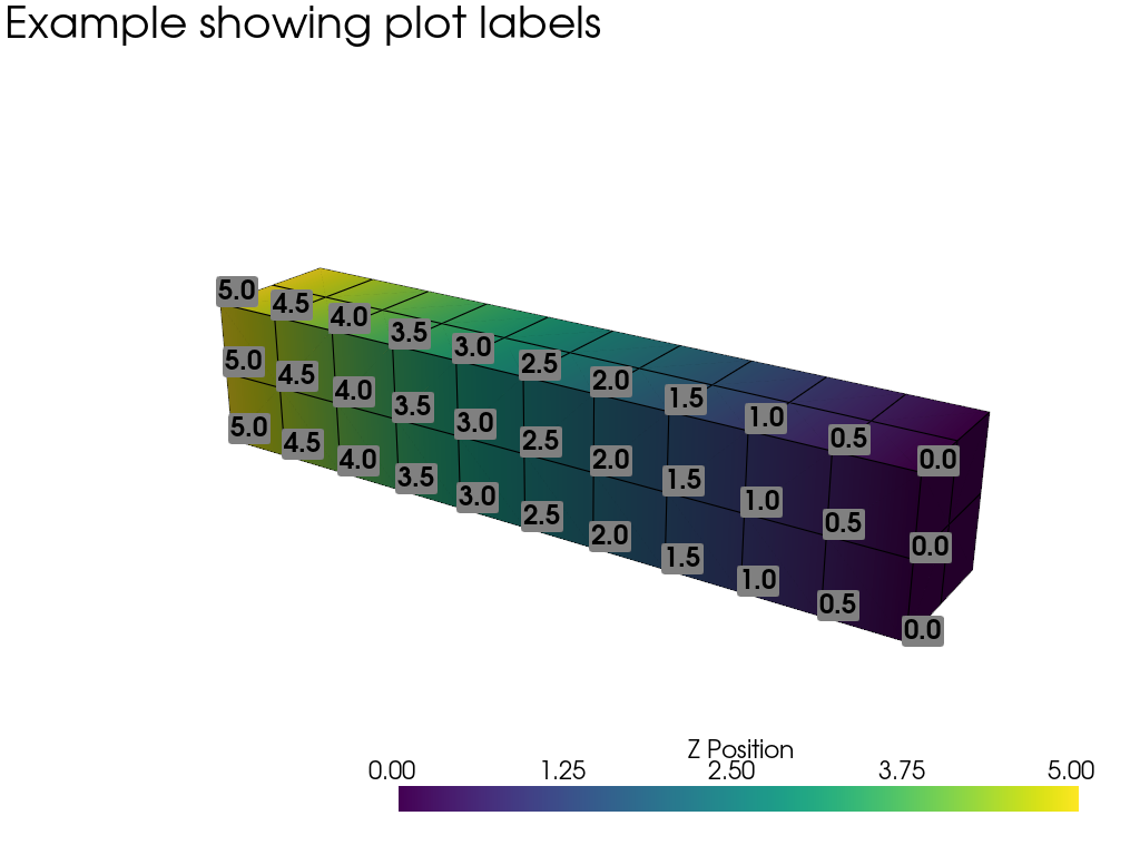
This example is similar and shows how labels can be combined with a scalar bar to show the exact value of certain points.

# Label the Z position
values = grid.points[:, 2]

# Create plotting class and add the unstructured grid
plotter = pv.Plotter()
# color mesh according to z value
plotter.add_mesh(grid, scalars=values,
                 scalar_bar_args={'title': 'Z Position'},
                 show_edges=True)

# Add labels to points on the yz plane (where x == 0)
mask = grid.points[:, 0] == 0
plotter.add_point_labels(points[mask], values[mask].tolist(), font_size=24)

# add some text to the plot
plotter.add_text('Example showing plot labels')

plotter.view_vector((-6, -3, -4), (0.,-1., 0.))
plotter.show()

Static Scene

Interactive Scene