Optional Features#
Due to its usage of numpy, the PyVista library plays well with
other modules, including matplotlib, trimesh, rtree, and
pyembree. The following examples show some optional features
included within PyVista that use or combine several modules to
perform advanced analyses not normally included within VTK.
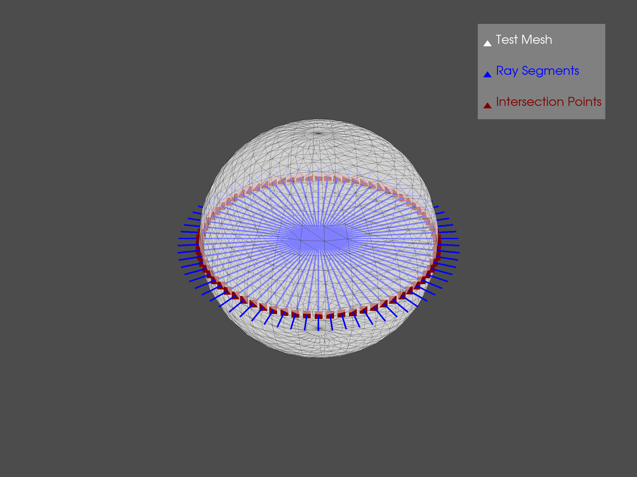
Vectorised Ray Tracing#
Perform many ray traces simultaneously with a PolyData Object (requires optional dependencies trimesh, rtree and pyembree)
from math import sin, cos, radians
import pyvista as pv

# Create source to ray trace
sphere = pv.Sphere(radius=0.85)

# Define a list of origin points and a list of direction vectors for each ray
vectors = [
    [cos(radians(x)), sin(radians(x)), 0] for x in range(0, 360, 5)
]
origins = [[0, 0, 0]] * len(vectors)

# Perform ray trace
points, ind_ray, ind_tri = sphere.multi_ray_trace(origins, vectors)

# Create geometry to represent ray trace
rays = [pv.Line(o, v) for o, v in zip(origins, vectors)]
intersections = pv.PolyData(points)

# Render the result
pl = pv.Plotter()
pl.add_mesh(
    sphere,
    show_edges=True,
    opacity=0.5,
    color="w",
    lighting=False,
    label="Test Mesh",
)
pl.add_mesh(rays[0], color="blue", line_width=5, label="Ray Segments")
for ray in rays[1:]:
    pl.add_mesh(ray, color="blue", line_width=5)
pl.add_mesh(
    intersections,
    color="maroon",
    point_size=25,
    label="Intersection Points",
)
pl.add_legend()
pl.show()
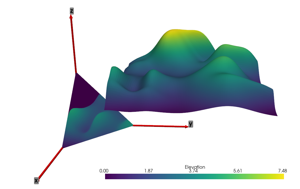
Project to Finite Plane#
The following example expands on the vectorized ray tracing example by
projecting the load_random_hills() example data to a triangular
plane.
import numpy as np
from pykdtree.kdtree import KDTree
from tqdm import tqdm

import pyvista as pv
from pyvista import examples

# Load data
data = examples.load_random_hills()
data.translate((10, 10, 10), inplace=True)

# Create triangular plane (vertices [10, 0, 0], [0, 10, 0], [0, 0, 10])
size = 10
vertices = np.array([[size, 0, 0], [0, size, 0], [0, 0, size]])
face = np.array([3, 0, 1, 2])

planes = pv.PolyData(vertices, face)

# Subdivide plane so we have multiple points to project to
planes = planes.subdivide(8)

# Get origins and normals
origins = planes.cell_centers().points
normals = planes.compute_normals(
    cell_normals=True, point_normals=False
)["Normals"]

# Vectorized Ray trace
points, pt_inds, cell_inds = data.multi_ray_trace(
    origins, normals
)  # Must have rtree, trimesh, and pyembree installed

# Filter based on distance threshold, if desired (mimics VTK ray_trace behavior)
# threshold = 10  # Some threshold distance
# distances = np.linalg.norm(origins[inds] - points, ord=2, axis=1)
# inds = inds[distances <= threshold]

tree = KDTree(data.points.astype(np.double))
_, data_inds = tree.query(points)

elevations = data.point_data["Elevation"][data_inds]

# Mask points on planes
planes.cell_data["Elevation"] = np.zeros(planes.n_cells)
planes.cell_data["Elevation"][pt_inds] = elevations

# Create axes
axis_length = 20
tip_length = 0.25 / axis_length * 3
tip_radius = 0.1 / axis_length * 3
shaft_radius = 0.05 / axis_length * 3
x_axis = pv.Arrow(
    direction=(axis_length, 0, 0),
    tip_length=tip_length,
    tip_radius=tip_radius,
    shaft_radius=shaft_radius,
    scale="auto",
)
y_axis = pv.Arrow(
    direction=(0, axis_length, 0),
    tip_length=tip_length,
    tip_radius=tip_radius,
    shaft_radius=shaft_radius,
    scale="auto",
)
z_axis = pv.Arrow(
    direction=(0, 0, axis_length),
    tip_length=tip_length,
    tip_radius=tip_radius,
    shaft_radius=shaft_radius,
    scale="auto",
)
x_label = pv.PolyData([axis_length, 0, 0])
y_label = pv.PolyData([0, axis_length, 0])
z_label = pv.PolyData([0, 0, axis_length])
x_label.point_data["label"] = [
    "x",
]
y_label.point_data["label"] = [
    "y",
]
z_label.point_data["label"] = [
    "z",
]

# Plot results
pl = pv.Plotter()
pl.add_mesh(x_axis, color="r")
pl.add_point_labels(x_label, "label", show_points=False, font_size=24)
pl.add_mesh(y_axis, color="r")
pl.add_point_labels(y_label, "label", show_points=False, font_size=24)
pl.add_mesh(z_axis, color="r")
pl.add_point_labels(z_label, "label", show_points=False, font_size=24)
pl.add_mesh(data)
pl.add_mesh(planes)
pl.show()