地形図

これは テクスチャを適用する の例と非常に似ていますが，地形メッシュの上にGeoTIFFからの航空画像をプロットすることに焦点を当てています．

from __future__ import annotations

import matplotlib as mpl
import matplotlib.pyplot as plt
import pyvista as pv
from pyvista import examples

まずは標高データと地形図を読み込むことから始めましょう．

# Load the elevation data as a surface
topo = examples.download_crater_topo().resample(0.5, anti_aliasing=True)
elevation = topo.warp_by_scalar()
# Load the topographic map from a GeoTiff
topo_map = examples.download_crater_imagery()
topo_map.to_image().resample(0.5, anti_aliasing=True, inplace=True)
topo_map = topo_map.flip_y()  # flip to align to our dataset

elevation

Header	Data Arrays
StructuredGrid Information N Cells 418701 N Points 420000 X Bounds 1.810e+06, 1.831e+06 Y Bounds 5.640e+06, 5.658e+06 Z Bounds 7.353e+02, 2.768e+03 Dimensions 700, 600, 1 N Arrays 1	Name Field Type N Comp Min Max scalar1of1 Points float64 1 7.353e+02 2.768e+03

先ほど読み込んだイメージを点検してみましょう．

mpl.rcParams['figure.dpi'] = 500
plt.imshow(topo_map.to_array())

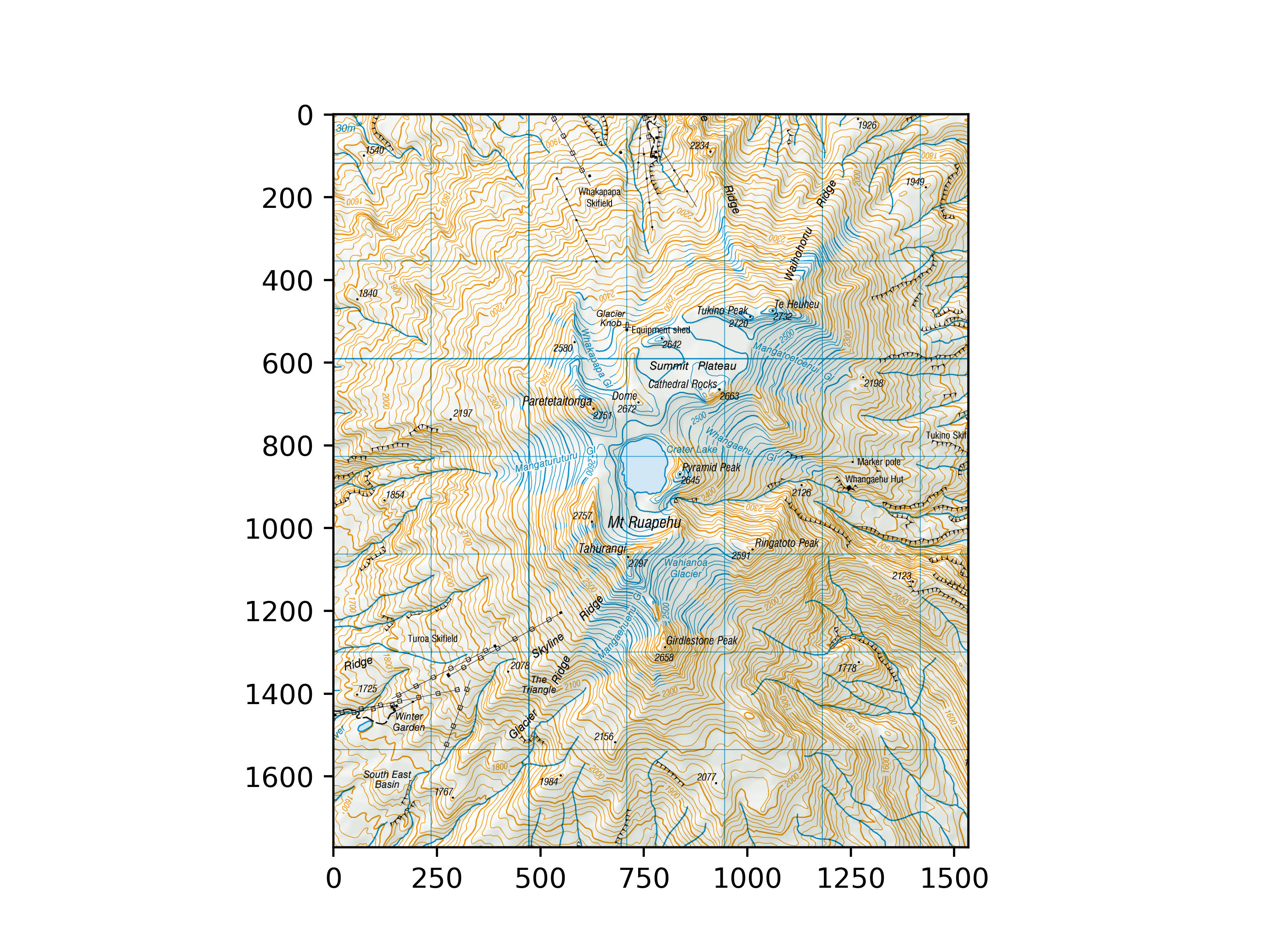
<matplotlib.image.AxesImage object at 0x7457a05b9a90>

サーフェスメッシュ(ここでは pyvista.StructuredGrid を使います)として地形メッシュをロードし， pyvista.read_texture() を使用して:class:pyvista.Texture としてイメージをロードしたら，次のようにイメージをサーフェスメッシュにマッピングできます．

# Bounds of the aerial imagery - given to us
bounds = (1818000, 1824500, 5645000, 5652500, 0, 3000)
# Clip the elevation dataset to the map's extent
local = elevation.clip_box(bounds, invert=False)
# Apply texturing coordinates to associate the image to the surface
local.texture_map_to_plane(use_bounds=True, inplace=True)

Header	Data Arrays
UnstructuredGrid Information N Cells 110369 N Points 57064 X Bounds 1.818e+06, 1.825e+06 Y Bounds 5.645e+06, 5.653e+06 Z Bounds 1.379e+03, 2.768e+03 N Arrays 2	Name Field Type N Comp Min Max scalar1of1 Points float64 1 1.379e+03 2.768e+03 Texture Coordinates Points float32 2 0.000e+00 1.000e+00

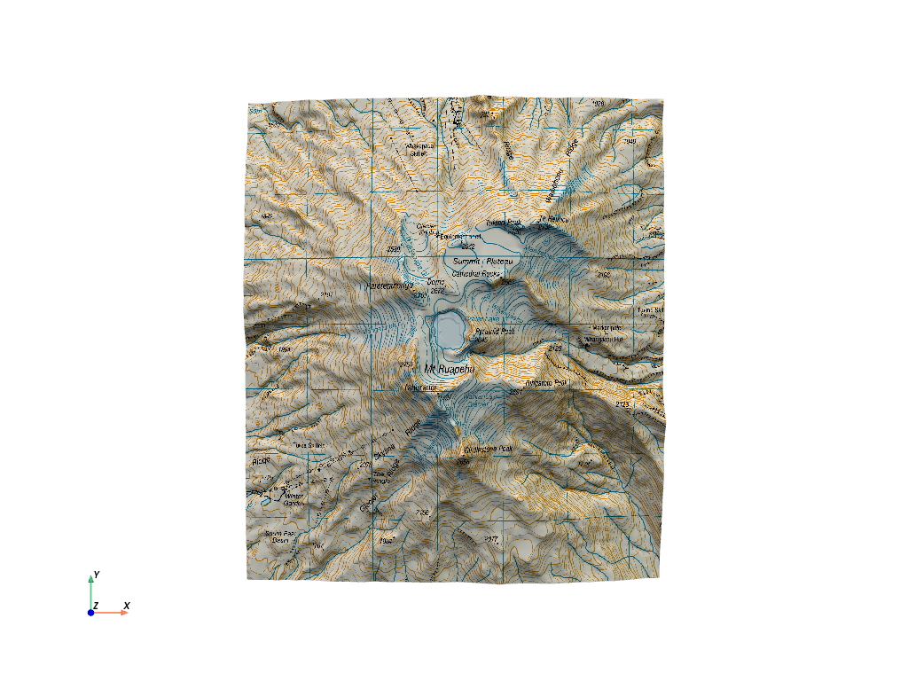
表示します．イメージが予想どおりに調整されていることに注意してください．

local.plot(texture=topo_map, cpos='xy')

スタティックシーン

インタラクティブなシーン

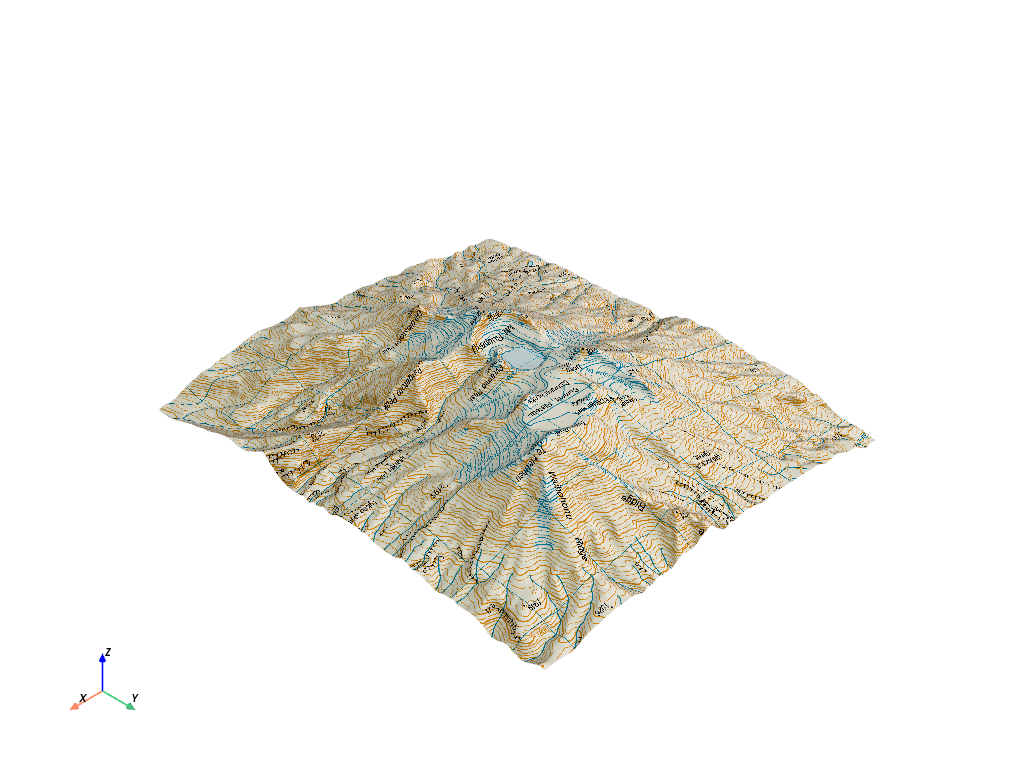
これが3 D遠近法です．

local.plot(texture=topo_map)

スタティックシーン

インタラクティブなシーン

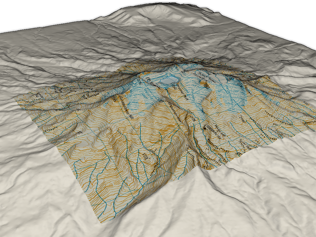
また，周辺領域を抽出し，テクスチャマッピングされた局所的な地形と外部領域をプロットすることによって，領域全体を表示することもできます．

# Extract surrounding region from elevation data
surrounding = elevation.clip_box(bounds, invert=True)

# Display with a shading technique
pl = pv.Plotter()
pl.add_mesh(local, texture=topo_map)
pl.add_mesh(surrounding, color='white')
pl.enable_eye_dome_lighting()
pl.camera_position = pv.CameraPosition(
    position=(1831100.0, 5642142.0, 8168.0),
    focal_point=(1820841.0, 5648745.0, 1104.0),
    viewup=(-0.435, 0.248, 0.865),
)
pl.show()

スタティックシーン

インタラクティブなシーン

Tags: plot